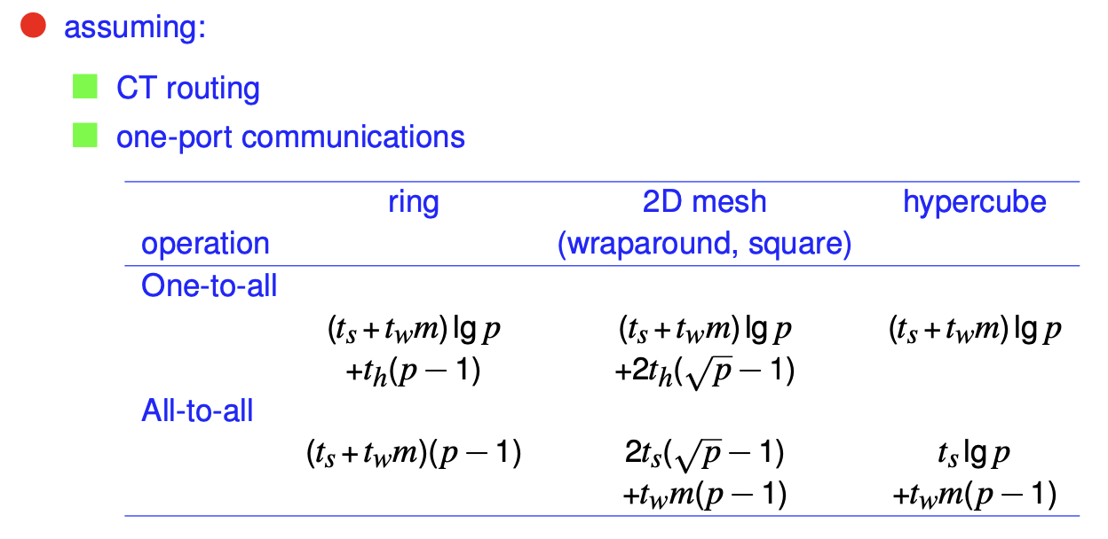
Shared Memory Address

Reference :

  • Introduction to Parallel Computing, Edition Second by Vipin Kumar et al
  • The Australian National University CECS

Shared Memory Hardware

Uniform Memory Acccess Shared Address Space with cache: 보통 UMA와 같지만 로컬 캐시를 가지고 있음

NUMA with cache: 보통 NUMA와 비슷함. 프로세서, 캐시, 메모리 한그룹이 묶여있고 이 그룹이 Interconnection Network을 통해서 연결되어 있음.

Shared Address Space Systems

  • 만약 로컬 메모리에 대한 접근이 원격 접근보다 가격이 싸다면 (즉 NUMA) 보다 싸다면 Shared Address Space Systems가 알고리즘에 포함되어야 함.
    • 어떻게, 운영체제가 호환되는지는 다른 문제임
  • 보통 공유 주소 공간을 가지고 있는게 프로그래밍 하기 쉬운이유가, 읽기 전용의 시스템은 그냥 순차적 프로그램 짜듯이 짜면됨. 다란 읽기/쓰기 같은경우, 병행적 접근때문에 MUTEX 가 필요함.
  • 주요 프로그래밍 모델들은 쓰레드와 directive based (컴파일러에 해당 인풋을 어떻게 처리할지 지시하는 언어적 구조) 이다. (Pthreads and OpenMP)
  • 동기화는 락과 관련된 메카니즘을 사용한다.

SASS with Shared memory computers

  • 공유 메모리는 전통적으로 메모리가 물질적으로 여러 프로세서들에게 연결되고, 모든 프로세서가 해당 메모리에 동일한 접근 권한을 가진곳에 사용되어 왔다.
    • 해당 방식은 UMA 라고 한다.
    • SMP는 원래 Symmetric Multi-Processor라 하여 모든 CPU들이 동일한 운영체제 성능을 (인터럽트나 다른 시스템콜 등) 가진것을 칭했는데, 요즘은 Shared Memory Processor의 축약어이다.
  • 분산 메모리 컴퓨터는 각 메모리의 다른 부분이 물질적으로 다른 프로세서와 연결되어 있음에 차이점이 존재한다. 이 distributed momory shared address space computer를 NUMA 시스템이라 한다.

멀티프로세서에서의 캐시

여러장의 데이터들이 여러 프로세서들에 의해 값이 변화된다.

  • 시스템 안의 각각의 물리적인 메모리 워드를 찾아낼 수 있는 주소변환 메카니즘, 그리고 여러 데이터들의 병행적 수행들이 잘 정의된 세만틱들을 가지고 있어야 한다.
  • 여러 프로세서들의 접근에 의한 캐시값의 일관성유지가 필요함.
  • 몇 기기들은 공유 주소 공간 메커니즘까지만 관여하고 일관성은 시스템이나 유저레벨의 소프트웨어에 일임한다.

Cache/memory Coherency

  • 매모리 시스템은 다음 사항들을 지키면 일관적이다
    • 실행된 순서대로 (Ordered as Issued) : 즉 한 프로세서가 읽고 수정하는동안, 다른 프로세서가 해당 값은 수정하지 않을때 (읽기는 가능)
    • 쓰기 전달 (Write Propagation): p1 reads, p2 writes, then p1 should have value of p2.
    • Write Serialization: 다른 프로세서들이 볼때 두 프로세서가 두 쓰기를 실행한 순서를 정확히 알고 있다면.

Cache Coherency Proctocol

캐시 일관성(Cache Coherence)

Invalidate Protocol: P0 P1이 같은 값을 읽었는데 P0가 값을 바꾸면, 해당 메모리와 이 값을 읽은 P1에게 이 값은 Invalidate되었음을 알려주는 방식 (이 값 쓰지마라) - 보통 이 방식을 사용

Update Protocol: P0 P1이 같은 값을 읽었는데 P0가 값을 바꾸면, 메모리와 P1이 가지고 있는 해당값을 업데이트 해줌.

비교:

  • 업데이트 프로토콜의 경우 같은 단어에 대한 여러 쓰기는 (거의 동시 읽기) 여러 쓰기 브로드캐스트s 를 필요로 한다. 이에 비해 Invalidate는 단 하나의 initial invalidation을 필요로 함.
  • 업데이트 프로토콜의 경우 여러 복수단어들의 캐시 블록들에게 각각의 캐시 블록 (라인)에 쓰여진 각각의 값들은 브로드캐스트 되어야 한다. 즉 한 블록에 한 단어만 보낼수 있음 (즉 여러 n 값들은 n번 보내져야 함). 반대로 invalidate only require one line.
  • 업데이트 프로토콜의 경우 한 프로세서가 한 값을 쓰고, 이 쓰여진 값이 다른곳에서 읽혀지는데 걸리는 지연시간이 더 적다. (즉 invalidate에 비해 값이 쓰여지고 읽혀지는 지연이 짧다는말)

False Sharing

두 프로세서는 같은 캐쉬라인에서 다른 부분을 수정함.

Invalidate의 경우 핑퐁된 캐시 라인들을 이용한다.

Update의 경우 로컬로 읽지만, 프로세서간의 업데이트 트래픽을 많이 발생시킨다.

다음 사항들을 병력 프로그래밍이나 시스템을 디자인 할때 항상 염두해야한다

  • 캐시라인 사이즈, 길수록 좋다
  • 캐시 라인 사이즈를 고려한 데이터 구조의 alignment

Implementation of Cache Coherency

  • 조그만 스케일의 버스 기반 기기들의 경우
    • 한 프로세서는 반드시 쓰기 invalidation을 브로드캐스트 할 수 있도록 버스에 대한 접근 할 수 있어야 한다.
    • 경쟁하는 두 프로세서들의 경우, 먼저 버스에 접근을 얻는 프로세서가 해당 데이터를 invalidate 한다 (즉 먼저 오는 프로세서의 값을 사용하는것)
  • 캐시 미스의 경우 데이터의 최신 카피를 위치해야 한다.
    • write-through cache 의 경우 쉬움
    • Write-back cache의 경우, 각 프로세서들의 캐시는 버스를 감시하며 데이터의 최신 카피가 있다면 반응한다 (snoop - 감시)
  • 읽기의 경우 다른 카피들이 해당 블록을 캐시했는지 알고싶어한다 (즉 해당 블록이 사용중인지)
    • write-back cache가 버스에 detail을 넣을지 말지 결정하기 위해서라던지
    • 태그를 이용해서 공유 status를 통해 관리한다
  • 프로세서 멈춤을 최소화하기
    • 태그들의 복사나, 혹은 inclusive cache 를 여러개 갖던지 하는 방식으로

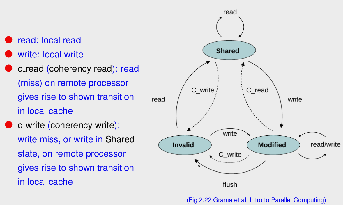
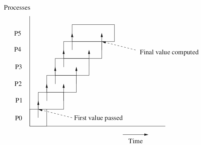
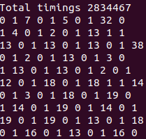
위 그래프와 아래 값들의 변화를 주의해서 살펴본다.
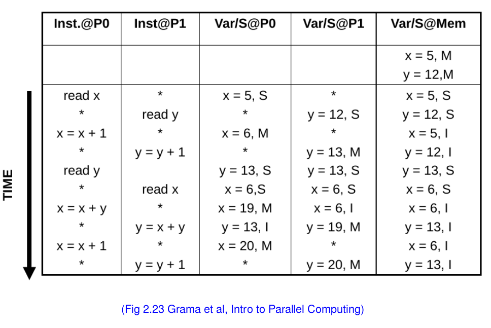
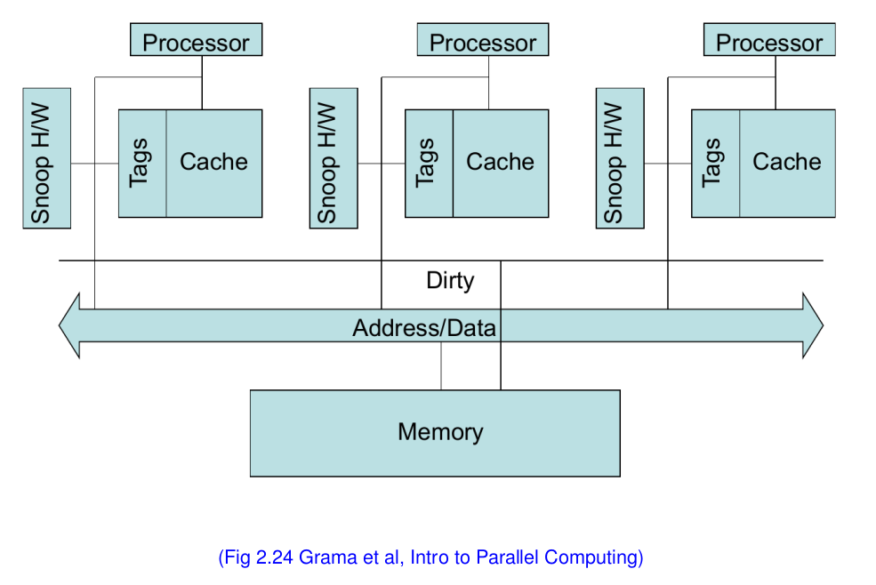
스누피 캐시 시스템

  • 모든 캐시들은 모든 변화를 브로드캐스트 한다
    • 버스나 링 위상의 interconnects에 쉽게 적합할수 있다 (implement)
    • 그러나 확장성이 재한되어 있다 (8개 이하).
  • 모든 프로세서들의 캐시들은 interconnect port의 변화를 감지한다 (관심있는 부분만)
    • 관련 프로토콜의 상태 다이어그램을 통해 태그들이 업데이트 된다.
  • 하드웨어 감시는 읽기가 한 더러운 카피를 가지고 있는 캐시블록에 대해 읽기가 실행되었으며, 이 행위가 버스 컨트롤에서 데이터를 빼내고, 관련 태그를 S로 바꾸었음을 알아차릴 수 있다. (예를 들어)

Directory Cache-Based Systems

디렉터리 기반 일관성 구조는 캐시 블록의 공유 상태, 노드 등을 기록하는 저장 공간인 디렉터리를 이용하여 관리하는 구조이다 - presence bitmap을 전역 메모리와 함깨 이용하여 각각의 메모리 블락이 어느 캐시에 위치하고 있는지를 디렉터리에 저장하는 방식.

이에 반해 디렉터리 기반 구조는 어떤 노드에서 해당 캐시 블록의 복사본을 가지고 있는지를 알고 있기 때문에 특정 노드에만 요청을 하게 된다. 따라서 브로드캐스트가 불필요하게 되어 대역폭이 상대적으로 작아도 된다. 이 때문에 64개 이상의 프로세서를 가지는 대규모 시스템에서는 디렉터리 기반의 캐시 일관성 프로토콜을 사용하는 경우가 많다.

이 디렉터리는 메모리와 붙어 있는데 공유 메모리의 경우 디렉터리가 따로, 로컬 메모리를 이용하는 경우 각각의 로컬 디렉터리를 사용한다.

  • 쉬운 프로토콜은 다음과 같을것이다
    • shared: 프로세서들은 블락 캐시를 가지고 있고, 메모리 값은 최신화를 유지한다
    • Uncached: 어느 프로세서도 카피를 가지고 있지 않는다 (즉 뺴서 저장하고 하지 않음)
    • Exclusive: 오직 한 프로세서만 (주인) 카피를 가지고 있고, 메모리에 있는 값은 옛날 값이다.
  • 공유되고 깨끗한 캐시 블록에대해 쓰기/읽기 미스와 쓰기는 다음과 같은 사항을 반드시 지켜야 한다
    • 이 블록에 대한 현 상태를 체크하기 위해 디렉터리 주소를 처음에 참조해야한다 (즉 directory entry를 먼저 refernce해서 상태 체크 해야함)
    • 그후에 entry의 상태와 presence bitmap을 업데이트한다
    • presence bitmap에 있는 해당 프로세서들에게 적절한 상태 업데이트 소식을 전달한다.

디렉터리 기반 시스템의 문제점

디렉터리 저장의 메모리 요구량

특정 데이터 접근 방법에 따른 퍼포먼스 차이

presence bitmap을 어떻게 관리할것인지 (복사? 꼭?)

어떻게 presence bitmap에 존재하는 모든 프로세서들에게 invalidation을 보낼것인지

  • MESI 프로토콜 출처
    • 캐시 메모리의 일관성을 유지하기 위해서 별도의 플래그(flag)를 할당한 후 플래그의 상태를 통해 데이터의 유효성 여부를 판단하는 프로토콜이다.
    • 데이터 캐시는 태그 당 두 개의 상태 비트포함한다.
    • 멀티프로세서 시스템에서 캐시 메모리의 일관성을 유지하기 위해 메모리가 가질 수 있는 4가지 상태를 정의한다.
      • Modified(수정) 상태 : 데이터가 수정된 상태
      • Exclusive(배타) 상태 : 유일한 복사복이며, 주기억장치의 내용과 동일한 상태
      • Shared(공유) 상태 : 데이터가 두 개 이상의 프로세서 캐쉬에 적재되어 있는 상태
      • Invalid(무효) 상태 : 데이터가 다른 프로세스에 의해 수정되어 무효화된 상태

Coherency Wall - 캐시 일관성의 한계및 단점

  • 인터커넥트는 로직 서킷들에 비해 50배나 넘는 에너지를 소모함
  • 각각의 invalidation을 위해 브로드캐스트 메세지를 필요로 하는 프로토콜의 경우
    • 에너지 소비는 O(p), overall cost = O(P^2)
    • 네트워크의 지연을 일으키기도 하다
  • 디렉터리 기반 프로토콜은 같은 데이터를 들고 있는 곳에만 메세지를 보낸다
    • 훨씬 확장성이 높으며 가벼운 데이터 공유를 가진다 (가진 애들끼리만 대화 하니까)
    • 이외는 모두 안좋다 잘못된 direction으로 인한 오버헤드도 발생함
    • 한 캐시 라인당, 비트 벡터의 길이가 a 라 하면 O(a^2) 의 공간 소모
  • false sharing은 어느 경우라고 트래픽을 낭비하는 모습을 보여줌
  • Atomic instructions 메모리 시스템의 동기화를 LLC (Last level cache) 까지 낮추는데 비용이 각각 O(p)

정리

  • 캐시 일관성은 실행 순서, 쓰기 전달, 쓰기 순차 세개의 요소를 가지고 있다
  • 두가지 방식을 가지고 있는데
    • 브로드캐스트/스눕: 중소 규모의 인트라 칩, 그리고 작은 인터 소켓시스템에 적합
    • 디렉터리 기반: 대중 규모의 인터 소켓 시스템에 적합
  • False sharing: 잠재적인 퍼포먼스 문제가 있음 (특히 캐시 라인이 길어질수록)
  • 대규모의 인트라 칩 시스템의 경우 일관성은 보통 운영체제나, Message Passing 프로그래밍 모델을 이용한다.

Message Passing Interface 2

MPI-1

  1. Fixed process model
  2. point-to-point communications
  3. collective operations.
  4. communicators for safe library writing
  5. utility routines

MPI-2

  1. Dynamic process management.
  2. one-sided communications
  3. cooperative I/O

Dynamic Process Management

  • MPI - 1 had a static or fixed number of processes
    • Cannot add nor delete processes
    • The cost of having idle processes may be large.
  • Some applications favour dynamic spawning
    • run-time assessment of environment
    • serial applications with parallel modules
    • scavenger applications.

CAUTION: process initiation is expensive, hence requires careful thought.

MPI-2 Process Management

  1. Parents spawn children
  2. Existing MPI applications can connect
  3. Formerly independent sub-applications can tear down communications and become independent.

Task Spawning - MPI_spawn();

  1. It is a collective operation over the parent process’ communicator.
  2. info parameter: how to start the new processes (host, architecture, work dir, path).
  3. intercomm and errcodes are returned values.

Communicators

  • MPI processes are identified by (group, rank) pairs.
  • Communicators are either infra group, or
    • inter group : ranks refer to processes in the remote group.
  • Processes in the parent and childern group each have thier own MPI_COMM_WORLD
  • Send and Recv have a destination and a inter/infra communicator.
  • Possible to merge processes or free parents from children by MPI_Intercomm_merge() and MPI_Comm_free().

One-sided Communications

For traditional MP, there is an implicit synchronisation - it may be delayed by asynchronous message passing.

In One-sided Communications,

  • One process specifies all communication parameters.
    • Data transfer and synchronisation are separate.
  • Typical operations are put, get, accumulate. MPI_put()

MPI-2 Remote Memory Access (RMA)

  • Processes assign a portion (or window) of their address space that explicitly expose to RMA operations. MPI_Win()
  • Two types of targets
    • Active target RMA: requires all processors that created the window to call MPI_Win_fence() before any RMA operations is guaranteed to complete.
      • One-sided communication: no process is req to post a recv.
      • Cooperative in that all processes must synchronize before any of them are guaranteed to have got/put data.
    • Passive target RMA: only requirment is that originating process places MPI_Win_Lock() and MPI_Win_Unlock() before and after the data transfer.
      • Transfer is guranteed to have completed on return from unlock.
      • Known as one-sided communication.
  • Potential unsync can be avoided by locks or mutexes.

MPI-2 File Operations

  • Positioning: explicit offset, shared pointer/ individual pointers
  • Synch: blocking/non-blocking (async)
  • Coordination: collective / non-collective
  • File types:
    • is a datatype made up of elementary types; MPI_Int()
    • allows to specify non-contiguous accesses.
    • can be tiled. s.t. process writes to block of the file.

MPI-IO Usage

  • 각 프로세서는 자신의 데이터를 따로 파일에 쓸수 있다
  • 프로세서들은 하나의 파일로 데이터를 추가 할 수 있다. (로그파일 형식) - 한 파일 포인터 사용
  • 프로세서들은 협력해서 하나의 큰 매트릭스를 파일에 쓸수 있다
    • 파일을 타일 하기 위한 파일타입 생성
    • 각가의 포인터를 이용
    • 모음 명령어를 이용하여 데이터 셔플링 가능케 함
  • 병렬 파일 시스템이 사용될수 있지만 그냥 평범한 파일 시스템으로 보일 수 있음

Simple MPI I/O

각 개인 포인터를 이용한 협력 파일 명령어. 각각의 프로세서의 메모리가 할당된 파일 타일에 데이터를 넣는 형식

  • MPI_File_Open() 을 이용하여 커뮤니케이터와, 각 개인 포인터와 공유 파일 포인터를 생성함
    • Info parameter 는 성능 조절, 특이 케이스 핸들링등에 대해 파일에 공유
  • 각각의 읽기 쓰기는 포지셔닝을 필요로 하는데 이는
    • MPI_File_Seek; …Read() —> 개인 파일 포인터 이용
    • MPI_File_Read_at; —> 해당 오프셋에서 직접적으로 읽기
    • MPI_File_seek_shared; … read_shared() —> 공유 파일 포인터 이용. Seek_shared is collective.
    • 읽기 쓰기로 버퍼, 카운트, 데이터 형식을 specify 한다 (보통 send/recev 처럼)
    • MPI_File_close() is also collective.

MPI-2 and Beyond

  • MPI-2 는 많은 기능을 넣었는데 1의 기능보다 훨씬 느려졌고, 해당 사용 회사들의 기능들은 오랫동안 미완성이었음
  • MPI-3는 단방향 통신과 non-blocking collective 를 향상 시킴

Synchronous Computations

Reference: Barry Wilkinson, Michael Allen - Parallel Programming_ Techniques and Applications Using Networked Workstations and Parallel Computers (2nd Edition) -Prentice Hall (2004)

Barrier

  • A particular reference point for processors which no one can proceed until every processors (or stated number) get to the point.
  • Commonly when processes need to exchange data and then continue.
  • Once the last one has arrived, inactive processes are awakened.
  • Apply both shared memory, and message-passing systemss

Barrier - MPI

  • MPI_Barrier(MPI_Comm comm) is called by each process and return once everyone arrives.
  • Naturally synchronus, and message tags are not used.

Counter Implementation

Called a linear barrier as well. Counting the number of processes is handled by a single counter.

  • Implementations must handle possible time delays for eg. two barriers in quick succession.
  • There are two phases:
    • Arrival Phase : Send msg to master and stay inactive or idle as not all are arrived.
    • Departure Phase : Receive from master and released.

— Remember Send() is not the blocking (depend on the buffer size), but Receive() always do the blocking. Cost = O(p) for time and computation complexity

Tree-Based Implementation

  • Use of decentralized tree construction.
  • Arrival and Depature order is reversal as it supposed to be.
  • Since it is up and down, O(2 lg p) = O(lg p) for communication time.

Note: broadcast does not ensure synch in terms of a global time

Butterfly (Omega) Barrier

Pairs of processes sync at each stage as following

  1. 01 23 45 67 (4 has 4,5)
  2. 02 13 46 57 (4 has 4,5,6,7)
  3. 04 15 26 37 (4 has 0,1,2,3,4,5,6,7)

After the stages, every processes are synchronized and can continue. O(2 lg p) = O(lg p) for communication time.

Local Synchronization

It can be formulated for only essential synchronization among few processes, instead of being “wastefully” idle — In a mesh or a pipeline and only neighbours sync. Not using barriers, but ues Receive to communicate and idle certian processes to exchange its data.

DeadLock

It will occur using synchronous routines (or blocking routines without sufficient buffering) if both performs the send first to each other. In general, assign even-numbere in send first, odd-numbered in rece first coule bo a good solution.

MPI_Sendrecv() and MIP_Sendrecv_replace() —> deadlock prevent commands.


Data Parallel Computations

  • ease of programming
  • ease of increase to larger problems.
    1
    2
    3
    4
    5
    6
    7
    8
    9
    forall (i = 0; i< n; i++){
    a[i] = a[i] + k;
    }
    // In SIMD, those particularly designed for these, implicitly has barrier itself
    // If MP computer using library routines, generally explicit barrier is required.
    // Following is an example
    i = myrank; // myrank is a process rank between 0 and n-1
    a[i] = a[i] + k; /* body */
    barrier(mygroup) // consider the barrier overheads as it may longer than its body

    Synchronous Iteration

Parallel started at the beginning of the iteartion, yet each processes cannot proceed to the next iteration unless all the assigined tasks in the iteration is completed.

Jacobi Iteration: all x are updated together.

  • guess X, and iterate while hope it converges.
  • In converges if tha matrix is diagonally dominant.
  • Terminates whin convergence is achieved (subtract of two is within the error tolerance)

야코비 방법

1
2
3
4
5
6
7
8
9
10
11
12
13
14
15
16
17
18
19
20
21
22
23
24
25
26
27
// Sequential 
for (i=0; i < n; i++){
x[i] = b[i]; //b[] holding the constants
}
for (iteration = 0; interation < limit; iteration++){
for (i = 0; i < n; i++){ // n number of rows and cols.
sum = -a[i][i] * x[d] // Jacobi method excludes itself.
for (j = 0; j < n; j++){ // each row summation iteration
sum = sum + a[i][j] * x[j] // summation of one row
}
new_x[i] = (b[i] - sum) / a[i][i] //a[i][i] cannot be zero
}
for (i=0; i<n; i++} x[i] = new_x[i] //data move
}
// Parallel
i = process_id;
x[i] = b[i]; // assign each process array for (iteration = 0; interation < limit; iteration++){
for (i = 0; i < n; i++){ // n number of rows and cols.
sum = -a[i][i] * x[j] // Jacobi method excludes itself.
for (j = 0; j < n; j++){ // each row summation iteration
sum = sum + a[i][j] * x[j] // summation of one row
}
new_x[i] = (b[i] - sum) / a[i][i] //a[i][i] cannot be zero
broadcast_gather (&new_x[i], new_x); //spread and gather data over processes
global_barrier();
for (i=0; i<n; i++} x[i] = new_x[i] //data move
}

Broadcast_gather expect all the processes to have matching routines. Hence further implementation must be made to avoid deadlocks whet each prcoss can stop once it met its tolerance (so each has diff num of iterations). It can be easily replaced with send and recv().

Analysis

Heat Equation

1
2
3
4
5
6
7
8
9
10
11
12
13
14
15
16
17
18
19
20
21
22
// Sequential Code
for (iter = 0; iter < limit; iter++){
for (i = 1; i < n; i++){
for (j = 1; j < n; j++){
q[i][j] = 0.25 * (h[i-1][j]+....);
}
}
for (i =1; i < n; i++){
for (j = 1; j < n; j++){
h[i][j] = g[i][j];
}
}
}
// Parallel Code
for (iter =0; iter < max_iter; iter++){
g = 0.25 * (w + x + y + z+);
send(&g, ...)
...
...
...
recv (&z, ...)
}

  • Block Partitioning: Each process generates and receives 4 messages each —> hence total of 8.
  • Strpi Partitioning: Two edges where data points are exchanged. Each edge generates and receives 2 messages —> hence total of 4.

In general, strip partition is best for a large startup time, and a block partition is best for a small start up.

For p ≥ 9, if above equation is fulfilled, the block partition has a larger communication time.

Safety & Deadlock

As it is unreliable to assume the internal buffer will be enough, there are two methods.

  1. Switching send and recv in different order as mentioned couple of times so far.
  2. Implement Asynchronus communication using ghost points.

Assign extra receive buffers for edges where data is exchanged. It is typically translated as extra rows and columns in each process’ local array (known as halo). In this buffer, asynchronus calls such as MPI_Isend() can be used.

Perfectly Parallel Models

Reference :

  • Introduction to Parallel Computing, Edition Second by Vipin Kumar et al
  • The Australian National University CECS

Granularity

  • Granularity: size of the tasks
    • Coarse grain: large tasks/many instructions
    • Fine grain: small tasks/few instructions
  • Metric = t_compute / t_communication
  • It may depend on number of processors.

Speedup

  • the relative performance between single and multiple processors
    • ⇒ S(n) = exe time on single / exe time on p = t_seq / t_par
  • t_seq should be the fastest known sequential algo; best parallel algo may be differernt
  • S_operation(p) = operation count rate with p / operation count rate on single
  • Linear speedup = max possible S(n) = p
  • if S(P) > P then
    • May imply the algo is not the best one, go and check the seq algo
    • May arise due to the unique feature of architecture.

Parallel Overhead

  • Factors that limit parallel scalability:
    • periods that not all p works + time when one p is active on seq parts
    • load imbalance
    • extra computations not in the seq code —> seq code in one p might be faster some cases
    • communication times

Efficiency and Cost

  • Efficiency: How well using the processors

$$E = t_{seq} / t_{par} / p = S(p)/p * 100%$$

  • Cost: parallel execution time * total num of p
    • Cost optimal = cost has same asymptotic growth as a func of input size as the fastest seq algo on a single processor

$$cost = t_{par} * p = (t_{seq}*p)/S(p) = t_{seq} / E$$

Adding n num on n processors

Adding n in a single core = n; adding n in n processor = lg(n). Therefore speedup = O(n/lg(n))

cost = number of p * time of execution = n * lg(n) = O(n lg(n))

Hence it is not cost-optimal

Scalability

Imprecise measure:

  • hardware: 하드웨어를 늘리면 퍼포먼스가 좋아지나?
    • 링, 크로스바, 하이퍼큐브 위상을 고려하고 프로세서에 무슨 변화를 줘야 하는지 고려
  • Algorithm: 사용하고 있는 알고리즘이 더 많은 프로세서와 accomodate 가능 한가?
  • Combined: 문제 크기 증가를 프로세서를 증가함으로써 accomodate 가능 한가?
  • 계산 사이즈를 배로 늘렸을때의 변화를 고려
    • N*N 매트릭스의 N사이즈를 두배로 늘리면, 더하기 계산의 비용은 4배지만 곱하기 비용은 8배로 늘어난다

Pipelining

Reference : Introduction to Parallel Computing, Edition Second by Vipin Kumar et al

Pipelinig

  • There are three types of pipelining;
    1. Adding numbers (type 1)
    2. Insertion Sort (type 2)
    3. Linear System back substitution (type 3)
  • Prblems that can be divided into a series of seq tasks that can be completed one after another.
  • Typical Scenario
    1. 독립된 문제가 한 개 이상 계산 될 예정일때 (Instruction)
    2. 각각 여러 계산을 필요로 하는 연결된 데이터들을 계산되어야 할때 (Graphics)
    3. 다른 계산에 필요한 작업이 그 계산이 필요로 하기전에 작업을 마칠수 있을때 (Software)

Type 1 - Adding number

  • Single Intance:

  • Multiple Instance:

Type 2 - Insertion Sort

Type 3 - Linear Equations

Back substitution —> passes calculated value to solve the other ones (like fibonacci).

Process i performs i sends and receives, i multiply/adds, one division/subtract and one final send

t_comm = (2i + 1) * (t_s +t_w) and t_comp = 2i + 2

Partition

Reference : Introduction to Parallel Computing, Edition Second by Vipin Kumar et al

Partitioning Strategies

  • Replicated Data Approach (No partitioning)
    • Each has the entire data but does a subset of computation.
  • Partition to different process (Most Common)
    • Domain Decomposition
    • Divide and Conquer
  • Partition of program func (Less Common)
    • Functional Decomposition

Partition to Diff Process

Use MPI_Scatter and MPI_reduce for Vector Addition

  • Root sends data to all processes (including itself)
  • MPI_Scatterv() —> scatters variable lengths. MPI_Allreduce() —> returns result to all processors

Domain Decomp via Divide-and-Conquer

  • For problems that can be recursively divided into smaller probs of the same type; such as summation.
  • The analysis for simple binary tree is as following

The Reduce and Scan Abstractions

  • 이미 프로세서들에게 파티션된 벡터들의 합이 이에 해당한다.
  • Reduce: Combines a set of val to produce a single value; mapping a binary tree communication pattern between processors.
  • Scan: performs a seq opreation in parts and carries along the intermediate results.

Scans

  • Replacs each element with the cumulative sum of all preceding elements (inclusive or exclusive)

    Parallel random-access machine

    1
    2
    3
    4
    5
    6
    7
    8
    9
    10
    11
    12
    13
    14
    15
    X = [0,1,2,3,4,5,6,7]
    Inc_Scan = [0,1,3,6,10,15,21,28]
    Exc_Scan = [0,0,1,3,6,10,15,21]
    //EX #1 - 8 val on 8 nodes.
    for (d=1; d < N; d ∗= 2)
    FORALL (k=0; k < N; k ++) IN PARALLEL
    if (k >= d)
    X[k] = X[k−d] + X[k];
    /***
    Ex #2 - Bucket Sort
    1. Assign one bucket to each processors
    2. Assign p small buckets to each processors --> can ues MPI_Alltoall()

    Ex #3 - Integraton (SPMD model using static distribution)
    --> Uneven workload, terminating point for small division is an issue.
  • The analysis for parallel bucket sort.

  • The worst case scenario: data is chunked at certain value —> same as the bucket sort problem?

Barnes Hut Algorithm

  • Algorithm —> It creates oct-tree
    1. Divide one cube into 8
    2. Delete if no needed
    3. sub-cube with more than 1 divided into 8 again.
    4. Continue untill each one has only one particle.
  • Scaling is O(n lg n)
  • Load balancing is likely be an issue for parallel code.

Parallel - Lab 2

Reference:

  • The Australian National University CECS

Timer Overhead vs Timer Resolution

Diffrences:

  • Timer overhead is the length of time it takes to call the timer function. The total time to run your program will be increased by this value multiplied by the number of times you call the timer.
  • Timer resolution is the period of time below which the timer will sometimes report a value of zero. It represents the smallest period that can accurately be measured by the timer.

Assess timer by calling it twice.

For timers that operate like clocks (real time or CPU time), the differences represent the change in the value of the clock between each call. The overhead is the average of the consecutively reported differences. The lowest measured values will be integer multiples of the resolution. If the overhead is less (or finer) than the resolution, then the measured overhead may be zero.

The above used gettimeofday()

The smallest non-zero is 1, hence the resoultion of the timer is 1us.

There are several zero valuse, hence the overhead or the timer is <1us.

The above used MPI_Wtime()

MPI_Wtick gives the resolution of 1e-09 which appears to agree the MPI_Wtime() hand calculation.

Blocking Behavior

The code fails because we have both processes wishing to send at the same time. If the message is small we see non-blocking behaviour since the message can be packed into the initial buffer (internal local system) —> Hence can store and move on to the next line of execution.

For larger sizes it fails because we see a transition from a non-blocking send to a blocking send when the message becomes too large. It stalls to find the receive() from the destination while the destination stalls and waits receive() as well.

Startup Time

Once the size reaches certian point, possibility of L3 Cache missing the data may cause decrease in the Bw; bw = 2.0 * length of words * sizeof(int) / time / 1e9 = GB/S

From the above results:
Latency = 4.42e-07s / 2 = 0.22 us ⇒ Ping Pong of empty messages average time.
Peak bandwidth ~= 1 GB/s

Routing

Reference : Introduction to Parallel Computing, Edition Second by Vipin Kumar et al

Routing and Communication Costs

Routing Mechanism - path msg takes

  • minimal: shortest path, Non-minimal: not shortest, for avoid network congestion.
  • Deterministic Routing: Unique path determined solely on the source and destination processor - ignore the state of the network.
  • Adaptive Routing : use information on the state of the network.

Review of SF and CT

Store and Forward (SF)

  • Common on early parallel
  • Forwards msg after the entire msg has been received and stored.
  • t_h is substantially less.

$$t_c = t_s + (m * t_w + t_h) * l \approx t_s * mt_w * l$$

Cut-Through Routing

  • msg is sent in fixed-length segments called flow-control digits or flits
  • Wormhole routing pipelines the flits through the network.
  • Uses less memory at the intermediate processor
  • msg header = l * t_h to arrive.

$$t_c = t_s + l * t_h * tw$$

  • cost is O(m+l) while O(m*l) for SF.

One-To-All Broadcast (OTAB) All-To-One Reduction (ATOR)

Ring or Linear Array

Recursive Doubling = 한곳으로 보내고 2명 2명이 2명에게 4명 4명이 4명에게….

Hence msg cab be broadcast in lg(p)

The destination node to each step to be sent must be carefully chosen to utilise the resources (avoid congestion on the network).

Reduction can be performed by reversing the direction and the sequence of communication —> will lead to the beginning node 0.

Mesh

  • Can regard each row and col of a square mesh of p nodes as a linear array or sqrt(p) nodes.
  • Perform like linear array on rows first, and do the same thing on the cols.
  • Hence 16 nodes (4*4) will be sqrt(16) = 4 phases in one-to-all broadcast. In 3D —> p^(1/3)
  • Reduction = same as linear array.

HyperCube

  • 2^d hypercube = d-dimension mesh with two nodes in each d.
  • Steps: d steps. 8 nodes (222) —> 3 steps.
  • The dimension is identified by the MSB, while the order of visiting dimension does not affect the communication —> Means no congestion.

Balanced Binary Tree

  • Hypercube OTA broadcast maps naturally onto it.

All-to-All Broadcast (ATAB) and Reduction (ATAR)

  • Used in matrix operations.
  • can be performed by p * OTAB or can be concatenated into one large message while traversing the network.

Linear Array and Ring

  • Each node = initial node. Use one way and pass it to the neighbour. First send urs then start to send the latest msg u got from the neighbour. Hence takes p-1 steps (need to receive 7 info in 8 nodes)

Mesh

  • Same as linear. Perform linear ATAB for rows and do cols.

Hypercube

  • hypercube = extension of mesh to log(p) dimensions. takes log (p) steps.

embParallel

Reference :

  • Introduction to Parallel Computing, Edition Second by Vipin Kumar et al
  • The Australian National University CECS

Embarrassingly Parallel Problems

  • 계산은 각각의 프로세서들에 의한 완전하게 독립전인 실행 부분으로 나뉘어질수 있다
  • 각각의 어플리케이션은 처치 곤란 병렬적이다
  • 데이터의 분포와 모음이 중요 이슈이다 - 비용이 많이 들거나, 중요하다
  • 대부분 마스터/슬레이브 접근방식을 사용한다 (p-1 speedup)

처치 곤란 병렬

망델브로 집합

Static Task Assignment

Each process needs to execute the procedure after being given the coordinates of the pixels to compute. Slave sends results back in groups which reduces the number of communication stratup times (for each message). — Note that master receives messages in any order.

Dynamic Task Assignment

Ideally, all processes must be busy; but we do not know the speed of each. Dynamic load-balancing can be achieved by a work-pool which get the works supplied when the process is idle. Each processors request a job when it finished its.

Summary

  • tasks do not need to communicate
  • non-tirvial but. providing input, aseemble the results, load-balance, scheduling, costing…
    • Static (low communication) vs dynamic + overdecomp (better load balance)
  • Monte carlo or ensumble simulations are a big use of computational power.
    • grid computing arose to solve this issue.

Message Passing

Reference : Introduction to Parallel Computing, Edition Second by Vipin Kumar et al

Message Passing Cost

  1. Startup Time (t_s): prepare the message (header, trailer, error correction information), execute the routing algorithm, establish an interface betw local node ane the router. —> Delay is incurred only once for a single msg
  2. Per-hop Time (t_h): after a msg leaves a node, takes a finite amount of time to reach the next node (=node latency). 어느 채널, 아웃풋 버퍼로 보내야 하는지 라우팅 스위치가 판단하는 동안 대기하는 시간과 직결된다.
  3. Per-word Transfer Time (t_w): if channel bandwidth is r words per second, t_w = 1 / r to traverse the link.

Store and Forward Routing - 전체 메세지 수신후 저장, 다음 노드로 전송

msg sizeof m, l links, t_h for header, t_w speed.

Total time = t_s + (t_h + t_w * m ) * l = t_s + mlt_w as t_h is comparatively small.

Packet Routing - Modification of SF.

Adv : 통신 자원 활용, 패킷 손실 (오류)로 인한 오버 헤드 감소, 다른 경로 선택 확률, 더 나은 오류 수정 기능.

이로 인해 장거리 네트워크 (인터넷 - 오류율, 홉 수, 그리고 네트워크 상태 변화 변수) 에 쓰임

Total Time = t_s + t_h * l + t_w * m where t_w = t_w1 + t_w2 * (1 + s/r)

각각의 패킷들이 다른 루트를 통해 전송 될수 있고, 잃어버린 패킷들의 재전송 때문에 지역/글로벌 네트워크에 많이 쓰임.

Cut Through Routing

  1. 모든 패킷이 같은 경로를 사용하도록 해서 라우팅 정보 오버 헤드를 제거
  2. 시퀀스 내 전달을 강제함으로 시퀀스 정보 제거
  3. 메세지 레벨 오류 정보 (패킷 레벨 말고)를 연관함으로 오류 검출 및 정정 오버 헤드 감소
  4. 병렬 시스템 오류율이 낮기 때문에, 값 비싼 오류 수정 체제대신 싼 오류 잠지 메커니즘 사용 가능

메세지를 flow control digits or filts 라는 고정 단위로 나눔 이는 패킷 오버 헤드를 미포함 하기에 패킷보다 작을수 있음

Tracer 가 목적지 노드에 먼저 도착후, 연결을 설정, 플릿이 차례대로 전송 (모두 동일한 경로, 중간에 기다림 없음 따라서 버퍼 미필요)

이 와 같은 특성으로 중간 노드에서 더 적은 memory and memory bandwidth and faster

Total Time = t_s + l * t_h + t_w * m

** 메세지가 작거나, 거리가 가까운 경우, 저장후전송과 컷쓰루 방식의 통신시간은 비슷하다.

제어 회로의 속도는 플릿 속도로 작동해야 하는데, 플릿 크기가 작으면 제어 회로 속도가 빨라지는데, 이는 라우터 설계에 상당한 어려움을 줌

플릿 크기가 크면, 내부 버퍼 크기가 증가하므로, 메세지 전송 대기 시간 (첫 시작노드) 이 늘어남.

요즘 플릿 크기는 4-32 바이트.

Total Time = t_s + l * t_h + t_w * m - 컷 쓰루 라우팅 공식

메세지 전송 비용 최적화를 위해

  1. Communication in Bulk: 조그만 메세지에 각각 t_s를 주느니, 큰 메세지 하나에 한번 주는것. 왜냐하면 클러스터/메세지 전달 시스템 같은 일반 플랫폼에서 t_s가 t_w 보다 훨씬 커서
  2. 데이터 볼륨 최소화: t_w로 인한 오버헤드 최소화를 위해, 통신되는 데이터 양을 줄이기
  3. 데이터 거리 최소화: 메세지가 통과해야 하는 홉 수를 최소화.

첫 1,2번의 경우 쉬우나 통신 노드 거리를 줄이는 (3)은 알고리즘 설계자에게 불필요한 부담을 줌. 왜냐하면

  1. MPI 에서 프로그래머가 물리적 프로세서에 프로세서들을 맵핑하는것에 권한이 조금 밖에 없음. 가까운 이웃간에 통신은 괜찮을 수 있으나, 전체적인 매핑에 손상을 줄 수 있기 때문
  2. 대부분의 아키텍처가 2단계 랜덤 라우팅을 이용하는데 (처음 한번 중간 한번). 이는 네트워크의 핫스팟과 부담감 (contention)을 줄여줌. 무작위 라우팅의 홉을 최소화 하면 이득이 없음
  3. 홉당 시간은 t_s 와 t_w * m 에 비하면 굉장히 작아, 홉당 시간을 무시해도 된다.

따라서 Total Time = t_s + t_w * m 으로 정리될 수 있다. —> 이 식은 혼잡하지 않은 네트워크에만 유효하다.

위 식은 런타임 예측 정확성과 독립적 알고리즘 설계에 중요한 영향을 미친다. 위의 식은 모든 노드간 통신에 같은 시간이 걸림으로, 완전히 연결된 네트워크에 해당함.

따라서 각 아키텍처 알고리즘 설계 하는 대신 비용을 생각한 알고리즘을 병렬 컴퓨터에 설계할 수 있게 한다.

물론 간소화된 공식으로 알고리즘을 설계 하면, 예측 정확도 손실이 발생하나, 홉당 시간이 굉장히 작다는 가정만 따른다면, 그 손실액은 미미하다.

For communication patterns that do not congest the network, the effective bandwidth is identical to the link bandwidth. However, for communication operations that congest the network, the effective bandwidth is the link bandwidth scaled down by the degree of congestion on the most congested link.

네트워크 정체 시키지 않는 대역폭은 링크대역폭. 네트워크 정체 시키는 통신의 경우 유효 대역폭은 가장 정체된 링크의 정체 정도에 따라 축소된 링크 대역폭. 이 값은 구하기 어려울 떄가 있음.

따라서 우리는 하한선을 이용하는데, link bandwidth = p/b (b = bisection width)

Communication Costs in Shared-Address-Space Machines

Cache Coherence에서 비용줄이기가 더 어려운 이유

  1. 메모리 레이아웃은 보통 시스템에 의해 결정된다. 프로그래머는 특정 데이터 아이템의 위치와, 순열 데이터 구조 최적화에 권한이 적음. 이는 이 공유 주소 공간 아키텍처에서 중요한데 로컬 및 원격 엑세스를 식별하기 어렵기 떄문. 로컬 과 원격 엑세스의 시간이 차이가 나면, 통신 비용은 데이터 레이아웃에 의해 크게 달라지기 때문.
  2. 유한 캐시 크기로 인한 캐시 스래싱 발생 가능. 사용 가능한 캐쉬보다 필요한 데이터가 클 경우, 특정부분이 덮어 쓰기 되어 여러번 엑세스 될 수 있음. 이 오버헤드로 인한 프로그램 성능이 크게 저하됨. 이 문제를 피하기 위해서는 작업 세트 크기를 최소화 한 실행 스케쥴이 필요. 멀티 프로세서의 경우 페널티가 심각해지는데, 이는 프로세서간 통신과 coherence 작업이 연관되기 때문.
  3. 무효화 프로토콜과 업데이트 작업은 수량화 하기 어렵다. 업데이트시 발생하는 트래픽의 경우 프로세서마다의 작업에 따라 확연히 달라지는데, 이 동시화된 데이터 갯수와 스케쥴은 프로그래머 권한 밖인 경우가 대부분.
  4. 공간적 지역성 (Spatial locality) 는 모델링 하기 어렵다. 캐쉬라인은 보통 한 단어(데이터)보다 길기에 여러개를 부르는데, 이에 따른 접근 시간이 단어마다 다르다. 이전에 불려진 데이터가 불려지는 경우 (다른것은 새거) 등은 프로그래머가 최소한의 제어를 가지기 떄문에, 프로그래머가 할 수 있는것은 순열 데이터 구조를 극대화 시켜 공간적 지역성을 최대화 하는것 밖에 없다.
  5. prefetching 은 데이터 엑세스와 관련된 오버헤드를 줄이는데 중요함. 컴파일러는 미리 로드를 진행할 수 있으며, 만약 자원이 충분할 경우 이에대한 오버헤드를 숨길수 있다 (현재 진행하는 작업을 느리게 하지 않으니, 몰래 미리 스윽 해놓기 때문에 오버헤드가 없는것) 이 와 관련된 사항은, 컴파일러, 레지스터, 캐쉬의 기능이므로 정확한 모델링이 어렵다.
  6. False Sharing 은 두 프로세서가 각각 사용하는 두 단어가 동일 캐쉬 라인에 있을수 있음 (공유하지 않아도) 이때 일관성 작업과 통신 오버헤드가 발생할수 있는데, 프로그래머는 이를 최소화 하기 위해 데이터 구조를 채우는 수밖에 없다.
  7. Contention in shared access 는 공유 주소 공간 기계에서 오버헤드를 발생시키는 주요 이유중 하나. 하지만 이는 실행 스케쥴의 기능이므로, 정확한 모델링이 어렵다 (스케줄링 알고리즘 문제가 아니니까). 계산해서 점근 추정값은 가능하나, 이 수치는 의미가 없다.

공유 주소 공간 머신의 모든 비용 모델은 이러한 오버 헤드를 고려해야 함.

Total Time = t_s + t_w * m

유한 캐쉬에서 발생하는 영향은 각 시스템마다의 다양한 캐쉬 사이즈로 인해 다르므로 무시됨

공간적 지역성의 최대화 (캐시 라인 효과)는 명시적으로 미포함

거짓 공유는 데이터 레이아웃과 같이 명령 스케줄의 기능

비용 모델은 공유 데이터 구조가 잘 채워져 있다고 가정하기에, 잘못된 비용 미포함

중복된 통신 및 계산을 설명하지 않음

Your browser is out-of-date!

Update your browser to view this website correctly. Update my browser now

×