Linear Regression

Reference:

1. An Introduction To Statistical Learning with Applications in R (ISLR Sixth Printing)
2. https://godongyoung.github.io/category/ML.html

Linear Regerssion is uesful tool for predicting a quantitative response. It is a good jumping-off point for newer approaches.

SLR

• It assumes there is a approximately a linear relationship between X and Y.
• hat denote the estimated value for an unknown parameter or coefficient or to denote the predicted value of the response.

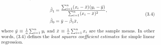
Estimating the Coefficients

• Wants to find parameter and coefficient as close as possible → use Least Squares

Assessing the accruacy od the Coeff Ests.

Population Regression Line: Generally not known.

• best linear approximation to the true relationship between X and Y.
• Each regression line may differ from this as the models are based on a separate random set of observations.

The purpose of using least square is to estimate caharacteristics of a large population.

If we estimate certain parameter based on a particular data set, it may overestimate or underestimate. However, observing huge amount of data and average will give us the exact value of it. Hence, treat the estimates as unbiased (such as hat values).

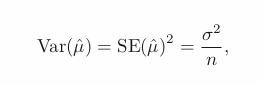
Stadarad Errors

• tells us the average amount that this estimate hat(mean) differs from the actual value of mean.
• can be used to conduct the confidence interval.
• can be used to perform hypothesis tests on the coeff.
  • t = hat(b1) - 0 / SE(hat b1)
  • if SE(hat b1) is small, it means the strong enough to reject null hypothesis
  • t measures the num of SD that hat(b1) is away from 0.
  • if no relationship, will have t-distrib with n-2 degrees of freedom.

p-value: indicates the unlikeness to observe the association between predictor and the response. Therefore, small p implies the associtaion.

The accuracy of the model

After we performs the hypothesis tests, want to quantify the extent to which the model fits the data by using: residual SE, and R^2 statistic.

1. Residual Standard Error (RSE):

   

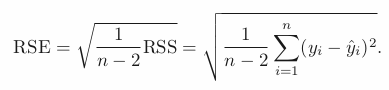
   • is an estimate of the standard deviation of error.
   • is the average amount that the response will deviate from the true regression line.
   • measure of lack of fit —> Small RES : well fit of data.

2. R squared: takes the form of proportion.

   

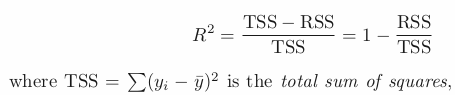
   • TSS measures the total variance in the Y and can be thought of as the amount of variability inherent in the response before the regression is performed.
   • RSS measures the amount of variability that is left unexplained after performing the regression.
   • Therefore TSS-RSS : var explained after the regression.
   • Hence, R-squared measures the proportion of var in Y that can be explained using X.
   • R-squared = correlation.

MLR

Important Qs

1. Is at least one of the predictors useful?
2. Do all the predictors help to explain Y, or is only a subset of the predictors useful?
3. How well does the model fit the data?
4. Given a set of predictor values, what response value should we predict, and how accurate is our prediction?

Relationship between Y and Xs

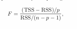
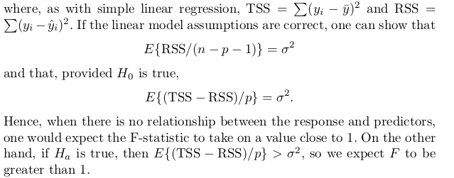
When n is large, F close to 1 might still provide evidence against null hypo.

Given these individual p-values for each variable, why do we need to look
at the overall F-statistic? After all, it seems likely that if any one of the
p-values for the individual variables is very small, then at least one of the
predictors is related to the response. However, this logic is flawed, especially
when the number of predictors p is large.

Hence, if H_0 is true, there is only a 5 % chance that the F-statistic will result in a p-value below 0.05, regardless of the number of predictors or the number of observations.

Decide on important variables

Variable Selection: AIC and BIC and Adjusted R-squared.

• Forward Selection: Start from Null. Fit p SLR and add to null model the variable that results in the lowest RSS.
• Backward Selection: Start from all. Remove the variable with the largest p-value (the least significant).
• Mixed Selection: p-values can become larger as more predictors. Hence. at some point conduct backward selection.

Model Fit

RSE and R-squared : the fraction of variance explained.

1. R-squared
   • In MLR, = Cor (y,hat(y))^2
   • In SLR, = Cor(y,x)
   • Will always increase with more variables - as it increase the accuracy of the model by adding more training data.
   • If the variable significant, it will bring substantial increase in the R-sq.
2. RSE
   • more variables can have higher RSE if RSS is small relative to the increase in p

Predictions

Uncertainty associated with prediction:

1. The inaccuracy in the coeff est. is related to the reducible error. Use confidence interval to determine the closness to true population regression plane.
2. Model Bias: potential reducible error that may come from the model. But we ignore and operate as if the model is correct.
3. Even if knows the TPRP, irreducible error makes impossible to accurately estimate the response value. Hence use prediction interval. It is always wider than CI as it both covers the irreducible and reducible.

Use CI for Y over a large num of cities. While use PI for Y over a particular city.

The coefficients and their p-values do depend on the choice of dummy variable coding —> use F-test.

Extensions

Important assumptions betwenn predictor and response are

1. Additive Assumption: the effect of changes in a predictor on the Y is independent of the values of the other predictors
   • Synergy Effect = Interaction Effect : spend newspaper and TV half can be better than putting all money in one place.
   • Use interaction term —> if X1X2 term has low p-val, then it means X1 and X2 (the main effects) are not additive each other (share the effect)
   • if we include an interaction in a model, we should also include the main effects, even if the p-val associated with their coeff are not significant.
2. Linear Relationship: using polynomid regression to accommodate non-linear relationship which still allows to use linear system.
   • Include polynomial functions of the prdecitors in the model to improve the fit
   • Unnecessary predictor makes the model wiggely, which casts doubt whether that additional variable makes the model more accurate.

Potential Problem

1. Non-linearity of the response-predictor relationships

   • Residual Plot - tool to identify non-linearity. Due to multiple predictors, plot residuals vs predicted (or fitted) y.
   • The presence of a pattern —> some aspect of the linear model.
   • If non-linear association, use non-linear transformations of the predictors such as log X, sqrt(X), and X^2

2. Correlation of error terms

   • If correlation exists, estimated SE will tend to underestimate the true SE. Hence, PI gets narrower, p-val is lower which could cause errorneously conclude that a parameter is statistically significant.
   • In short, lead unwarranted sense of CI in the model.
   • Time series data: Residual plot, if error terms are positively correlated, tracking in the residuals - adjacent resi may have similar valuse.

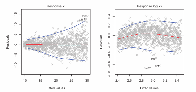
3. Non-constant variance of error terms

   • SD, CI, Hypothesis test rely upon this

   • heteroscedasticity: funnel shape in the residual plot.

   • Solution: transform results in a greater amount of shrinkage of the larger responses, leading to a reduction in heteroscedasticity.

     

4. Outliers

   • Usually has no effect on the least square fit. But has significant effect on RSE which is used for CI and p-values —> important for the interpretation of the fit. + R-sq declines as well.
   • Use studentized residuals: each residual / ESE. ≥ 3 is outlier
   • It may imply missing predictor, so be aware.

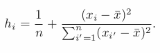
5. High-leverage points

   • Removing high leverage has more substantial impact on the least squares line than removing an outlier.

   • It may invalidate the entire fit —> better remove it.

   • Leverage Stat: ≥ (p+1)/n —> suspect

     

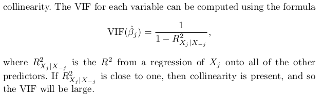
6. Collinearity

   • predictors are closely related. Use Contour plot of RSS for visual.

   • Small change in the data could cause the pair of coeff values that yield the smallest RSS, the smallest LSE, to move anywhere along the valley. It is a great deal of uncertainty in the coeff est.

   • It reduces the accuracy of the esitimates of the regression coefficients, hence, increases the SE of hat(predictor).

   • It reduces the t-stat hence affect the hypothesis test weak (the probability of detecting a non-zero coeff).

   • Use Variance inflation factor (VIF): value of 1 indicates the absence of collinearity. Exceeds 5 or 10 —> problematic amount of collinearity.