Statistical Learning

Reference:

1. An Introduction To Statistical Learning with Applications in R (ISLR Sixth Printing)
2. https://godongyoung.github.io/category/ML.html

Why Estimate f?

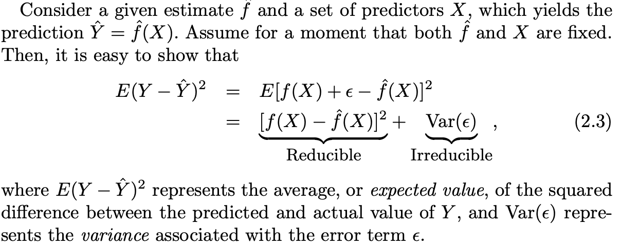
1. Prediction: hat(y) represents prediction of y.
   1. reducible error: imperfect estimate of hat(f) of f - can be fixed by using SL to estimate f.
   2. irreducible error: error introduced by random error term cannot be reducible no matter how well estimate the f. larger than zero:
      1. as there are some useful variables not considered in predicting y.
      2. There are unmeasurable variation that may change day by day.

Parametric Methods

• make an assumption about the functional form.
  1. stick to esitmating the chosen form instead of testing all of the others; know what u need.
  2. Uses the training data to fit or train the model. For linear → least squares.

Assuming a parametric ease the entire process compares to trying to fit the model into arbitrary forms. It may not match the true form of the function, which can be fixed by flexible model (it requires far more parameters though). But this flexible model can also be overfitting (follw the errors or noise too closely).

Non-parametric Methods

• Do not make explicit assumptions about the f form. seek an estimate of f that gets as close to the data points as possible.
  • Pros: potential to accurately fit a wider range of possible shapes for f (모양을 가정하지 않기떄문에)
  • Cons: large # of observations is required.

Wrong amount of smoothness may result in overfitting - as it does not yield accurate estimates.

Tread offs in flexi and interpreta

• IF interested in inference → more restrictive model is more interpretable. ⇒ difficult to understand how individual predictor is associted with the response.
• Interested in prediction: moderate flex and interpret is better due to the possibility of overfitting.

Supervised vs Unsupervised Learning

• Unsupervised: lack a response variable that can supervise our analysis.
  1. Cluster Analysis: whether the observations fall into relatively distinct groups → each group may differ.
     • Not be expected to assign all of the overlapping to their correct group (too crowded).

Will be covered in the different chapter.

Regression vs Classification

1. Quantitative - Numerical Values
   • regression Problems
2. Qualitative - K different classes or categories.
   • Classification Problems

The differene is vague. Both can be co-used in various methods. Although tend to select via type of response varaible (패러미터의 타입은 중요하지 않음).

Measuring the Quality of fit

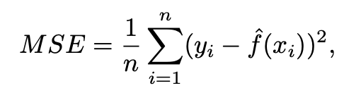
Measure of how well its predictions actually match the observed data. In the regression setting, it is MSE.

Interested in predicting unseen test observation (whether it is future event or not) which is not used to train the model. Consider Degree of freedom and MSE results for finding suitable methods.

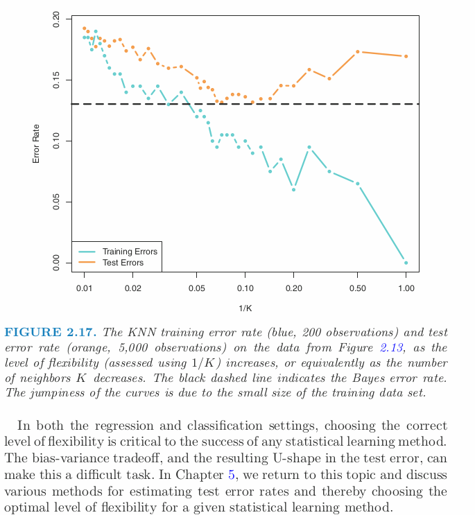
• we observe a monotone decrease in the training MSE and a U-shape in the test MSE. This is a fundamental property of statistical learning that holds regardless of the particular data set at hand and regardless of the statistical method being used.
• As model flexibility increases, training MSE will decrease, but the test MSE may not. When a given method yields a small training MSE but a large test MSE, we are said to be overfitting the data.

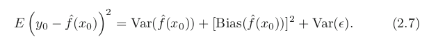
Bias-Variance Trade off

• Variance: amount by hat(f) would change if we used different training data set to estimate it. x의 변화에 민감하게 그래프가 꺾임. Least Square (straight line) has inflex, low variance.In general, more flexible methods have higher variance.
• Bias: error that is introduced by approximating a real-life problem. Linear regression (straight line cannot explain real life) results in high bias but also could estimate accurately via cases.Generally, flexible → less bias.

Classification Setting

equal = 1, inequal = 0

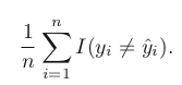
• Above equation computes fraction of incorrect classification = training error rate as computed based on our training data for the classification.

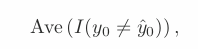
• Test error rate. A good classifier = one has small test error rate. = Misclassification error rate.

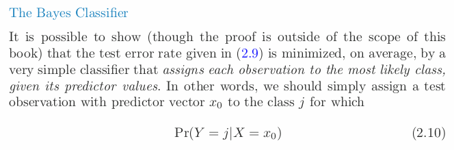
• Bayes Decision Boundary: line that assign each test data sets into categories it belongs to.
• It has the smallest error (in the population).
• In real life, not know the conditional distribution of Y given X. so impossible to use.

K-Nearest Negihbors

k-최근접 이웃 알고리즘

• attempt to estimate the conditional distribution then classify to get highest estimated probability.

1. Identify K points in Tr that are closed to x_0 represented by N_0.
2. Estimates conditional prob for class j as the fraction of points in N_0 whose response values eq j.
3. Applies Bayes Rule and classifies with the largest prob.

As K grows, the method becomes less flexible and produces a decision boundary that is close to linear. This corresponds to a low-variance but high-bias classifier.